Enable and use the compress scopes feature

Download python script

This example demonstrates how to enable and use the compress scopes feature introduced in the 24.05 release.

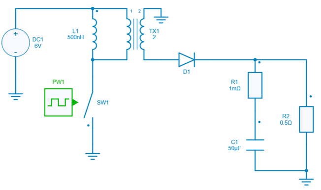
The circuit model used in this example is a flyback converter, which is directly loaded from the collection of design examples.

The main steps of this example are as follows:

Load Module, Project, and Design Example

This requires aesim.simba version 2024.05 or higher. Additionally, matplotlib.pyplot can be imported to view the curves and results.

Add a scope to the control square source

An output control probe is added to C1:

C1 = flybackConverter.Circuit.GetDeviceByName("C1")
for s in C1.Scopes: s.Enabled = True

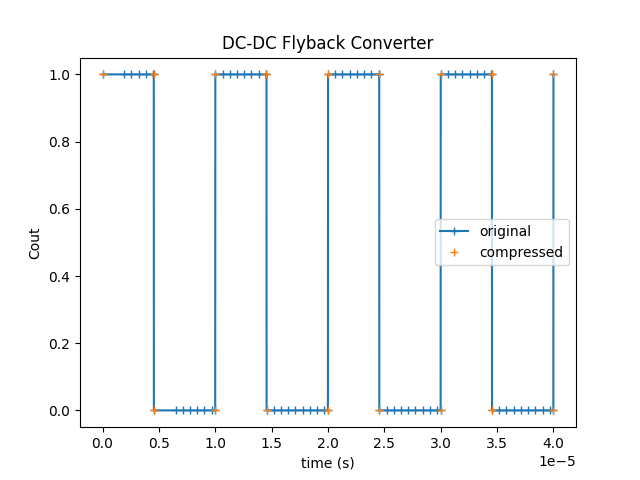
Run simulation and plot signals without the compression, then activate the compression and rerun the simulation

Activate the scope compression:

flybackConverter.TransientAnalysis.CompressScopes = True

When the scope compression is enabled, the job TimePoints vector is empty. Each signal has its own TimePoints vector:

Cout_signal = job2.GetSignalByName('C1 - Out')
Cout_with_compression = Cout_signal.DataPoints
t_with_compression = Cout_signal.TimePoints

Note: The control scope Cout does not have the same size (number of points) with and without the compression.

len(Cout_without_compression): 25981
len(Cout_with_compression): 81

py Cout_signal.TimePoints is the same as py job1.TimePoints when the scope compression is disabled.

Note: As the scopes have different sizes, they cannot be plotted with the same time vector, and the current vector job.TimePoints cannot be used to plot the compressed signal.

Results are shown below: