Using the Jupyter Notebook

This tutorial explores the usage of "Jupyter Notebook" with SIMBA python module.

Jupyter is a Free software, open standards, and web services for interactive computing across all programming languages.

Jupyter Notebook is also called "web-based interactive computing platform” and isn the original web application for creating and sharing computational documents. It offers a simple, streamlined, document-centric experience as it combines live executable code, equations, narrative text, visualizations, images, ...

More information could be found from Jupyter official website

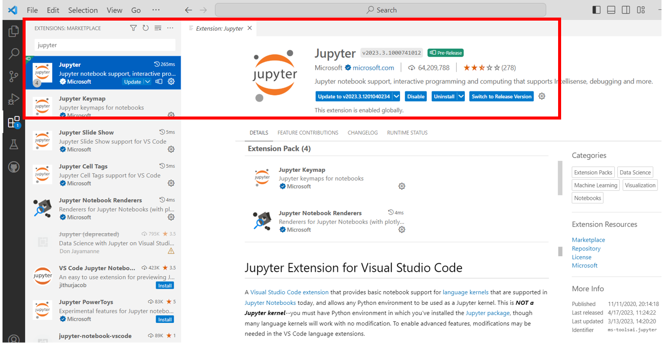
How to install Jupyter tool with Visual Studio Code

By using Visual Studio, click into the “extensions” tab and search the “jupyter” application.

Click on “Install” for allowing to create interactive document.

Files creation and cells manipulation

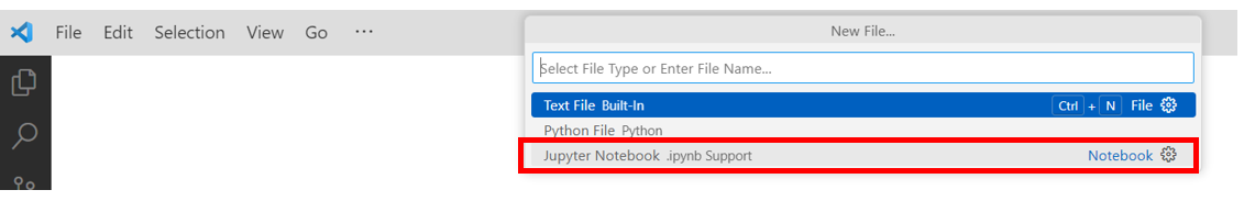
✔ Step 1: A new “Jupyter Notebook” file could be created by using the extension “.ipynb”.

Click on "File" tab --> "New File" and select "Jupyter Notebook"

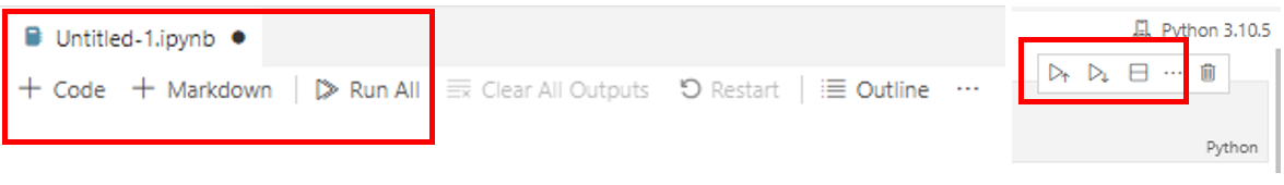
After clicking on the “.ipynb” extension, the new jupyter notebook file is shown as below:

A notebook file is structured by cells. A cell is the basic element of a Jupyter notebook: it can contain text formatted in Markdown format or code that can be executed.

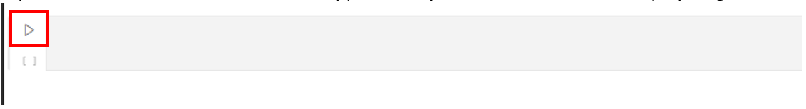
✔ Step 2: By clicking on “+ Code”, a new cell will appear that you can execute with the “play” tag: any python scripts could be inserted in this place

✔ Step 3: By clicking on “+Markdown”, a new cell will appear, but you cannot execute it, it is just for text and visualization. Any images, links, equations, pictures, texts could be inserted in this place.

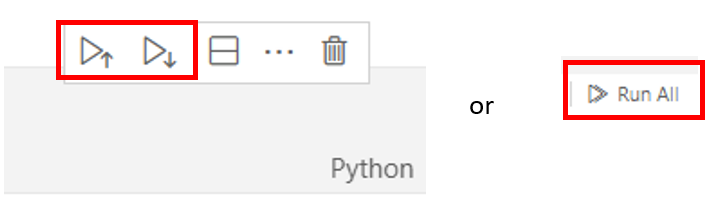
✔ Step 4: All the cells could be run by using the below buttons:

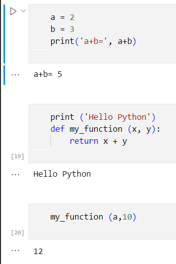
Cell with code

Let's create new cells including those below “python” scripts and run them. The results are highlighted as well.

Cell with markdown

What is markdown?

Markdown is a lightweight markup language which makes it easy-to-read and easy-to-write. Formatting elements are added to plaintext text documents to get formatted text (bold, italic, links, titles, images, mathematical formulas...). Thus, it can be used for creating websites, notes, documents, presentations, technical documentation, etc.

Markdown can be written in a file with a “.md” extension and then be easily converted into HTML or PDF file. More information could be found from Markdown official website.

Basic markdown syntax rules can be found directly here.

Let's observe the below example which shows how to implement markdown syntax:

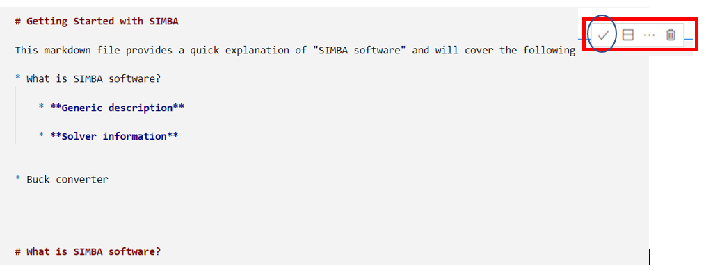
You can also edit the cell and modify its content. The final content will be:

SIMBA simulations, pre and post-processing with Jupyter Notebook

As mentionned above, cells in a jupyter notebook can be run independently: some of them can be dedicated to write some notes or plot drawings, other ones to run simple python code and other ones to run SIMBA through its python module.

This gives space run SIMBA simulation and to perform pre or post-processing using any python module.

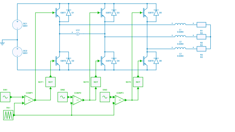
The example below deals with the sweep of modulation index $m$ depending on dc bus voltage $E$ for a three-phase-inverter.

✔ Step 1: Pre-processing

Let's compute the modulation index for different DC bus voltages to get the same AC voltage by using the expression:

$$m = \frac{2 U \sqrt{2}}{E \sqrt{3}}$$

Let's copy and paste the corresponding python code into a cell:

line_line_voltage = 300
fmod = 50
dc_bus_voltages = [800, 700, 600]
modulation_indexs = 2 * line_line_voltage * np.sqrt(2) / dc_bus_voltages / np.sqrt(3)

✔ Step 2: Load design and get elements to run simulations

In a new cell, let's load the project, the circuit and then get the circuit elements (voltage sources vdc1, vdc2 and modulation control blocks pwm) which are going to be modified:

project = ProjectRepository(os.getcwd() + R"\Three-phase-inverter.simba")
mycvs = project.GetDesignByName('three-phase-inverter')
vdc1 = mycvs.Circuit.GetDeviceByName('DC1')
vdc2 = mycvs.Circuit.GetDeviceByName('DC2')
pwms = [mycvs.Circuit.GetDeviceByName('SIN'+k) for k in ['1', '2', '3']]

✔ Step 3: Run simulations and store results

Simulation results will be stored in three different lists: time, line-line voltage u12and inductor current iL. Let's initialize these lists in a new cell:

res_time = []
res_u12 = []
res_iL = []

Now, let's run simba simulations for the different modulation indexs - which have been previously computed - with a for loop on the couple (DC bus voltage, modulation index). This can be done in a new cell or be added to the previous one. Note that at each iteration the results are appended to the python lists.

for dc_bus_voltage, modulation_index in zip(dc_bus_voltages, modulation_indexs):
    vdc1.Voltage = dc_bus_voltage / 2
    vdc2.Voltage = dc_bus_voltage / 2
    for pwm in pwms:
        pwm.Amplitude = modulation_index
        pwm.Frequency = fmod
    job = mycvs.TransientAnalysis.NewJob()
    status = job.Run()
    res_time.append(job.TimePoints)
    res_u12.append(job.GetSignalByName('U12 - Voltage').DataPoints) 
    res_iL.append(job.GetSignalByName('L1 - Current').DataPoints)

✔ Step 4: Post-processing

Let's load a new package, Bokeh, to plot results. This package provides different options than matplotlib

from bokeh.plotting import figure
from bokeh.io import show, output_notebook

Now, let's prepare two figures with zoom options, legends and labels to plot the AC line-line voltage and the current through the inductor.

# plot
TOOLTIPS = [
    ("index", "$index"),
    ("(t, val)", "($x, $y)"),
    ]

# figure 1
p1 = figure(plot_width = 800, plot_height = 300, 
           title = 'Line-line voltage',
           x_axis_label = 'time (s)', y_axis_label = 'Voltage (V)',
           active_drag='box_zoom',
           tooltips = TOOLTIPS)
# figure 2
p2 = figure(plot_width = 800, plot_height = 300, 
           title = 'Line current',
           x_axis_label = 'time (s)', y_axis_label = 'Current (A)',
           active_drag='box_zoom',
           tooltips = TOOLTIPS)

At last, let's plot the results with a FOR loop to iterate on the different results with a color variation:

green_color = 50
for time, u12, iL in zip(res_time, res_u12, res_iL):
    p1.line(time, u12, color=(0, green_color, 0))
    p2.line(time, iL, color=(0, green_color, 0))
    green_color += 100

output_notebook()
show(p1)
show(p2)

The results will be directly displayed into the jupyter notebook such as :

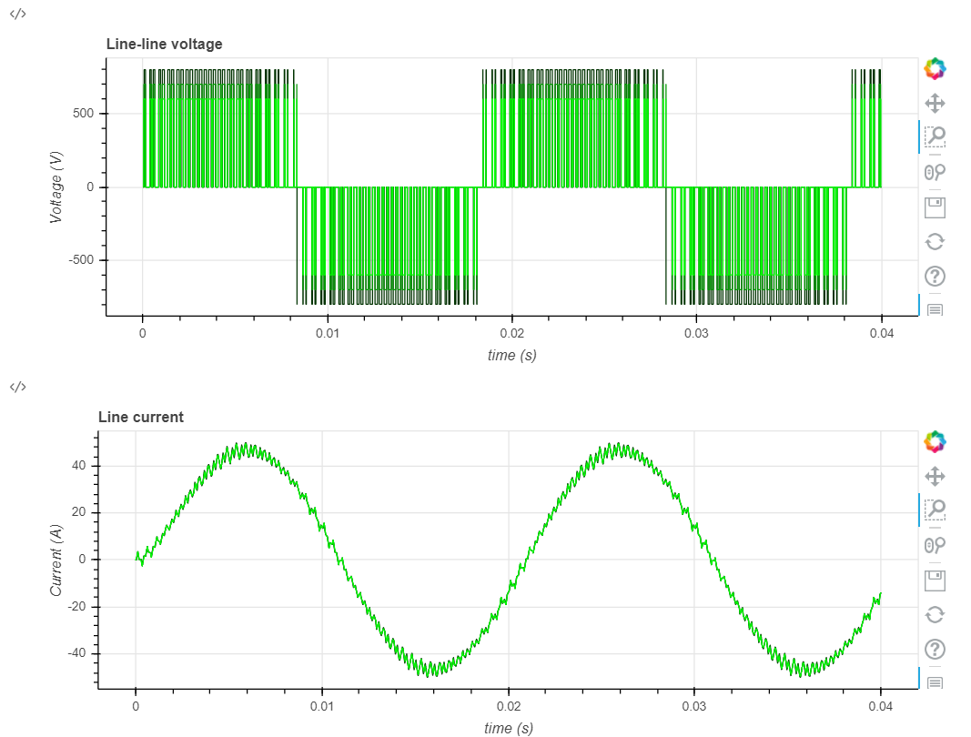
In that sense, any user can use python notebooks to run any mathematical equations, display graphs / pictures and calculate for example transfer function / body diagram, transient behavior….

This concludes this tutorial about the usage of "Jupyter Notebook" feature.