Example of optimization using Scipy Library
This python script proposes a simple example of optimization using Minimize() function of Scipy Library. The example considers an impedance adaptation circuit and the objective is to determine the load resistance which leads to the transfer of the maximum power.
How to Proceed
Create a Circuit
The model can be created in SIMBA GUI:
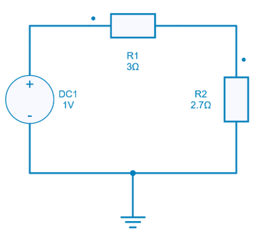
It can be seen that a voltage source with its internal resistance R1 supplying power to the load R2. Now, let us consider that R_1 has the fixed value of 3 Ω.
Write an Objective Function
To maximize the power delivered to the load, an objective function has to be defined with:
- the value of resistor R2 as a input,
- the computed value of the transferred power as an ouput.
Here are the main steps of this function:
- load the created model,
- apply value of resistor R_2,
- run the simulation,
- compute and return transferred power.
def objective_function(R_load):
    file_path = os.path.join(os.getcwd(), "max_power.jsimba")
    project = JsonProjectRepository(file_path)
    maximum_power = project.GetDesignByName('maximum_power')
    maximum_power.Circuit.GetDeviceByName('R2').Value = R_load[0]
    job = maximum_power.TransientAnalysis.NewJob()
    status = job.Run()
    Iout = job.GetSignalByName('R2 - Current').DataPoints
    power = Iout[-1]**2*R_load
    project.Save()
    return -power
Note
This objective function returns a negative power for the minimize() function of Scipy Python library, as the objective is to maximize the transferred power.
Use Minimize() Function of Scipy
The minimize() function is a part of the scipy.optimize module in the Scipy library, which provides tools for solving optimization problems, including both unconstrained and constrained optimization. The minimize() function is used to find the minimum of a scalar function of one or more variables, possibly subject to constraints. It employs various optimization algorithms to find the solution.
The syntax is as given below:
Parameters:
- fun: The objective function to be minimized. This function should accept a 1-D array (or list) of parameters as its first argument and return the scalar value of the objective function.
- x0: Initial guess for the optimization variables.
- args: Additional arguments to be passed to the objective function.
- method: The optimization algorithm to use. Scipy provides various methods like 'BFGS', 'CG', 'Nelder-Mead' also known as Downhill Simplex, 'L-BFGS-B', 'trust-constr' for steepest descent etc. You can choose the method based on the characteristics of your problem.
- bounds: Bounds for optimization variables. It can be either a sequence of (min, max) pairs for each variable or a single tuple (min, max) that applies to all variables.
- constraints: Constraint definitions, if any. Constraints can be specified as dictionaries or objects with a specific format depending on the constraint type.
Additionally, there are many other optional arguments for fine-tuning the optimization process, controlling convergence criteria, and more.
In this example, the method chosen is L-BFGS-B (Limited-memory BFGS with box constraints). Other methods can also be used for this example as per the user convenience.
The initial guess and bounds can be defined as:
initial_guess = np.array([2.7])
bounds = [(2.5, 3.5)]
result = minimize(objective_function, initial_guess, method='L-BFGS-B', bounds=bounds)
Example of results
For this example, a typical run can lead to the results below printed with 4 digits after the dot.
Of course, with a simple example, these results are closed to the theoretical value of 3 Ω. For other more complex problems, the initial guess as well the bounds can also be considered to explore a wider domain.