Closed Loop Design of an LLC Resonant Converter for a 3.3kW On-Board Charger Application

Download Simba Model

This example helps to understand how to tune the inner and outer loop of a controller of an LLC resonant converter using Simba and SmartCtrl. It can also use a python script which can be downloaded here to transform the data in an appropriate way (see below for more explanation).

The specifications of DC-DC Full Bridge LLC Resonant Converter for a 3.3 kW on-board charger applications are as below:

Inputs:
- $(V_{in})_{rated}$ = 400 V
- $(V_{in})_{min}$ = 390 V
- $(V_{in})_{max}$ = 410 V
Output:
- $(V_o)_{rated}$ = 420 V
- $(V_o)_{min}$ = 300 V
- $(V_o)_{max}$ = 420 V
- $(P_o)_{rated}$ = 3.3 kW
Resonant frequency: $f_{res}$ = 200 kHz

The complete design values can be obtained by following the design steps mentioned in LLC Converter Design example. In this case, the $Ln$ and $Qe$ values considered are 4 and 0.4 respectively.

The following steps need to be followed for tuning the inner as well as outer loop:

Set up the circuit to perform AC Sweep for inner loop.
Obtain and save the AC Sweep data in '.txt' format using python script mentioned above.
Open SmartCtrl to import the data for tuning the controller of inner loop.
Perform the simulation for inner loop after obtaining the controller values from SmatCtrl. It is to ensure the proper working of inner loop with the selected values.
Set up the circuit to perform AC Sweep for outer loop after closing the inner loop.
Close the outer loop again by obtaining the controller data from SmartCtrl.
Finally, validate the complete model by performing the closed loop simulation.

AC Sweep set up for inner loop

After obtaining all the values for the required specifications, the circuit has to be simulated in open loop to check its performance. The controlled input here is the relative frequency (control block 'C1') whose value is such that the output should be set at the "nominal output voltage". Here it is kept at 0.8 and hence the frequency of operation will be 160 kHz (= 0.8 x 200 kHz) to get the nominal output voltage.

AC_SweepInner

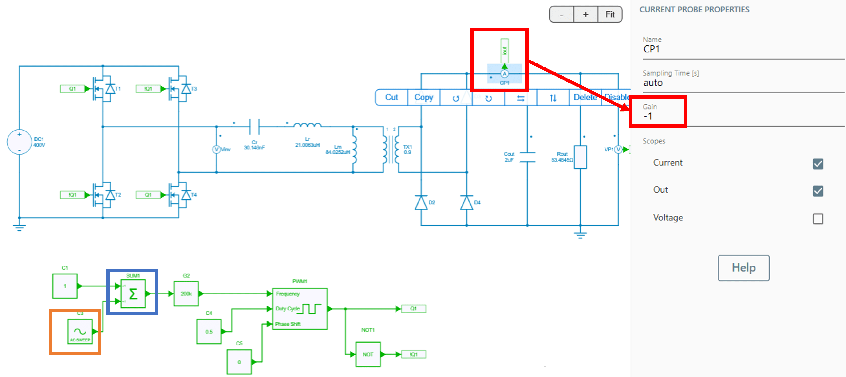
AC Sweep Test Bench has to be setup in Simba GUI. Before proceeding for AC Sweep Test Bench, make sure to add an 'AC SWEEP' block in GUI as shown in figure above. Since, the objective here is to obtain a plot for control-to-output transfer function, the perturbation has to be injected at the control input. Consequently, the AC SWEEP block is added to the control block using SUM block. For inner loop, the output here is current, so make sure to enable the scope which measures the output current. In this case, the scopes of 'CP1' is enabled which measures the unfiltered output current.

Note

The gain of the scope is set at -1 to depict the inverse relation between the control input and the output. For ZVS operation, the converter has to be operated in inductive region where the output decreases with the increase in frequency of operation.

Now, go to the Test Bench in Simba GUI, and set up an AC Sweep Test Bench with the parameters as below:

testbench1

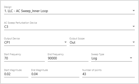
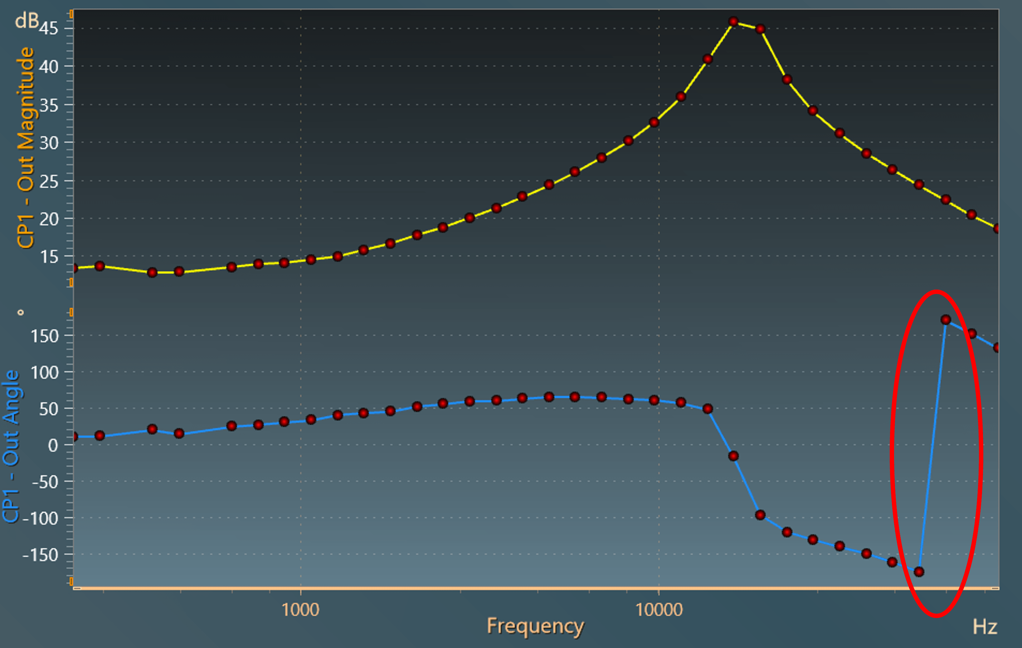
The above parameters can further be tuned by the user to get better waveform. The result of the AC Sweep can be analyzed by running the AC Sweep simulation which is as shown in figure below:

ACSweep1_result

Obtain the AC Sweep data in '.txt' format

The above AC-Sweep data can be exported either in .csv format or in .png format from the result window of Simba GUI.

Warning

The format of angle supported here is from -180° to +180° as highlighted in the figure above. Since SmartCtrl uses .txt format and angle from 0° to 360° format, one can use a python script to generate the data in the required format.

The following line of python code is used to convert the angle data in modulo 360°:

phase_sim1 = list(map(lambda p : p if p<65 else p-360, phase_sim1))

To generate the data in .txt format, pandas python library can be used as shown in below code (where 'tab' separator is used to differentiate the different columns):

df = pd.DataFrame({'Frequency': frequency_sim1, 'Amplitude': mag_sim1, 'Phase': phase_sim1 })
SweepInner_txt = "SweepInner.txt"
df.to_csv(SweepInner_txt, sep='\t', index=False)
print(f"Data has been exported to {SweepInner_txt}")

Tuning of inner loop using SmartCtrl

The file generated in above step can directly be imported in SmartCtrl to tune the controller. The steps mentioned below must be followed:

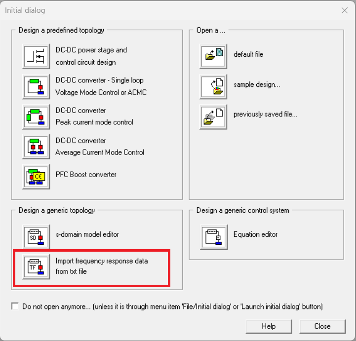
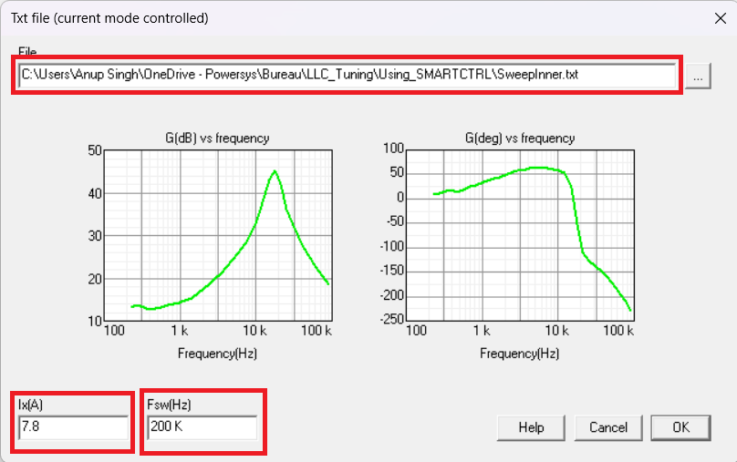
Launch SmartCtrl, 'Initial Dialog' window will be popped up and click on 'Import frequency response data from txt file' option at the bottom left of this window.

SC1

In the next window, select 'Current mode controlled' and click 'OK'. Further , provide path to the AC Sweep data in .txt file and give input as 7.6 in 'Ix(A)' tab, 200K in 'Fsw(Hz)' tab and click on 'OK'. This is because the output current is 7.8 Amperes at the nominal output voltage and the switching frequency is 200 kHz.

SC2

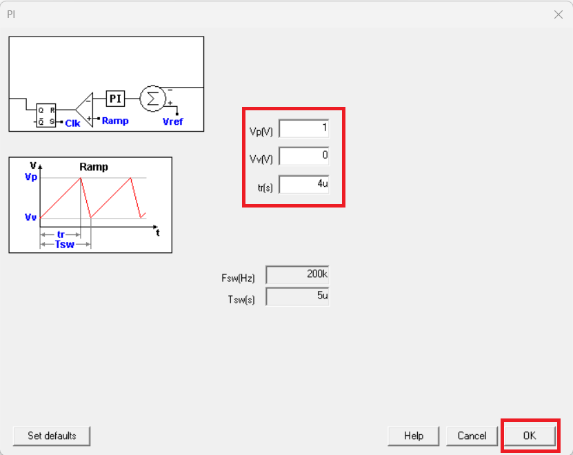
Further in next window, select 'Current sensor' under 'sensor' tab, put its 'Gain' as '1' and click 'OK'. Consequently, 'Compensator' tab will be enabled and select 'PI' option from the drop-down menu. In this 'PI' window, write '1' in Vp(V) tab, '0' in Vv(V) tab, '4u' in 'tr(s)' tab and click 'OK'. It will take back to the previous window.

SC3

Now, in this window, select 'Set...' tab which will show the solution map in a graph in white region, choose any point in the solution region and click 'OK'. This is the initial solution that is selected and it will take back to the previous window.

SC4

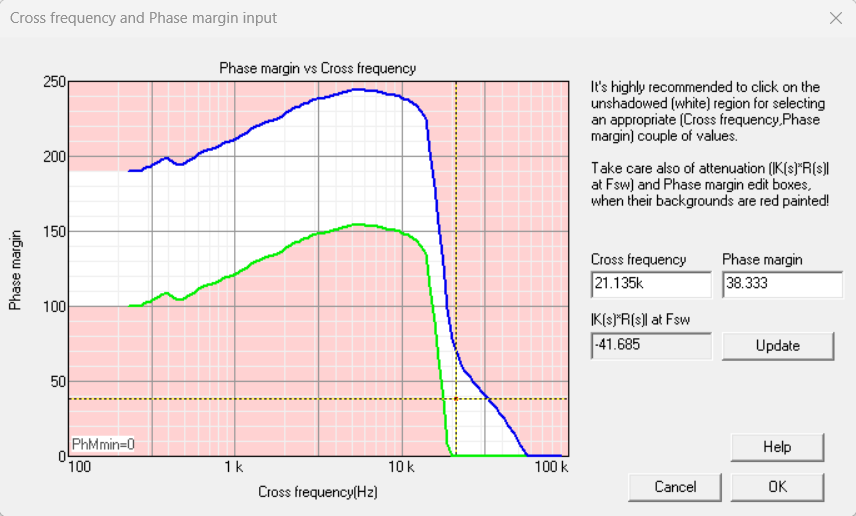
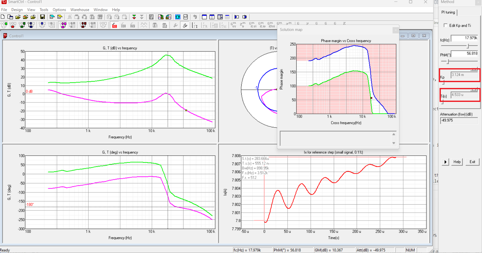
Finally, click 'OK' to reach to the final solution window where frequency and time domain analysis can be observed for the selected point in the solution map. In this case, initially, the selected value is Kp = 3.124m and Ti(s) = 4.533u which gives the Ki value ( $\frac{Kp}{Ti(s)}$ ) as 689.168 which is to be entered in the controller of inner loop.

SC5

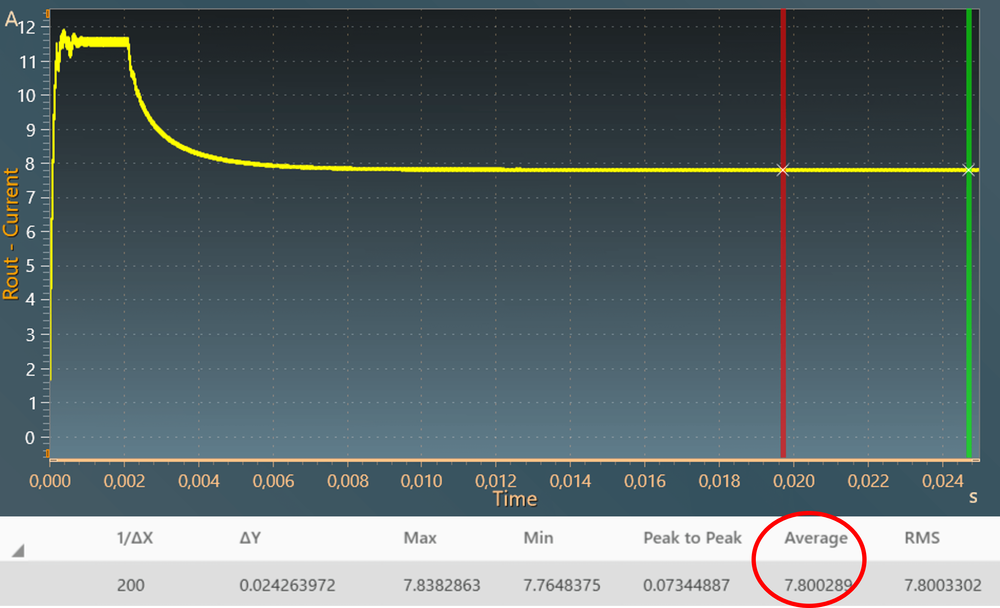
With this value of the controller, close the inner loop and check the results. It can further be tuned and final value selected here is Kp = 0.75m and Ki = 75 as shown in the attached model in design '2. LLC - Inner Loop' whose design and result are shown below:

design_innerloop

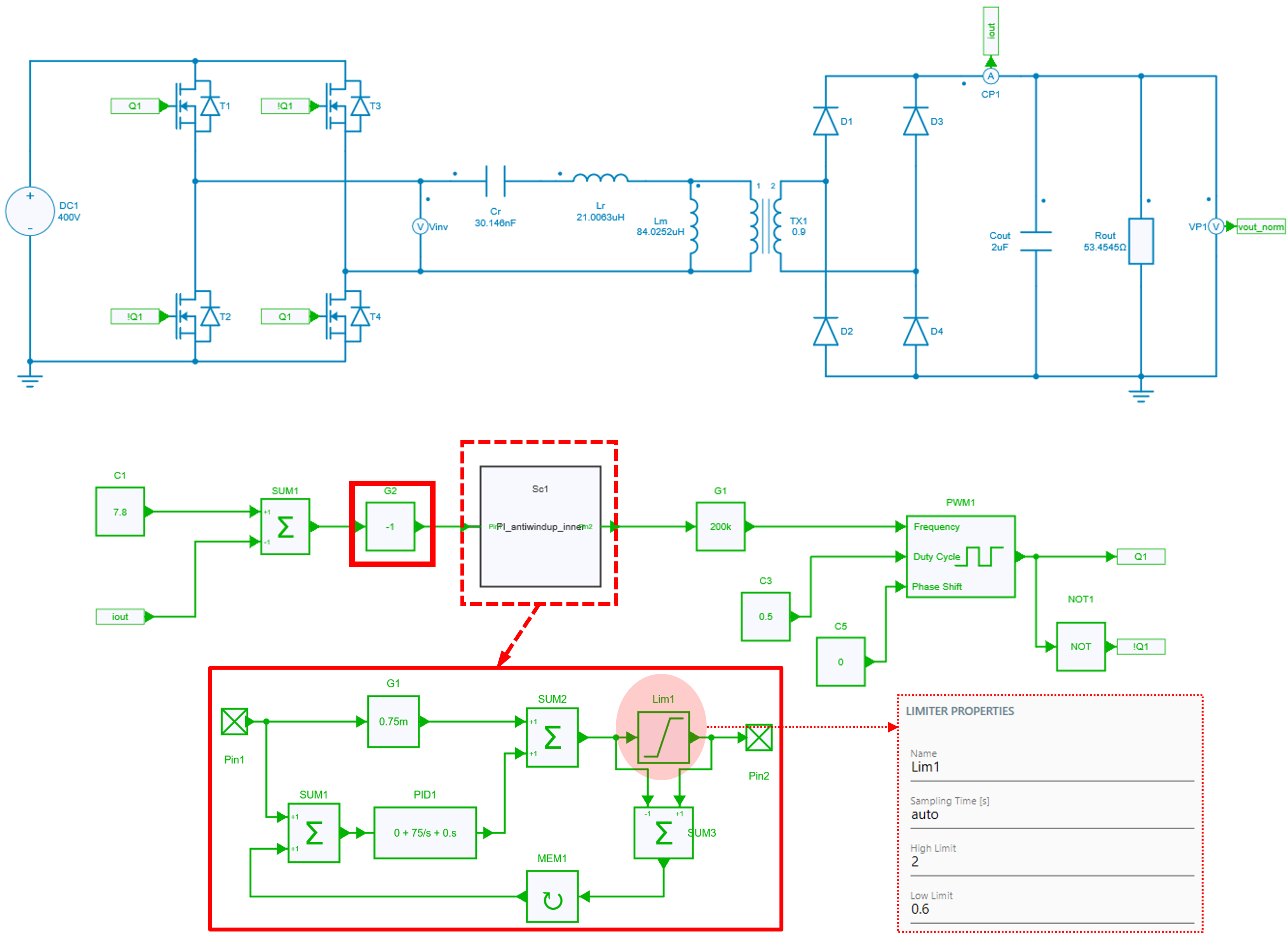
Note 1

It can be noted that there is a limiter connected to the 'PID block' to make an anti-windup PI controller whose lower limit is 0.6 and higher limit is 2. This should be there to make integrator work in the desired range of operation. Removing the limiter could allow controller operation in the capacitive region which would lead to the loss of ZVS operation.

Note 2

The negative gain of the sensor is now placed before the controller.

result_innerloop

AC Sweep set up for outer loop

The AC Sweep outer loop can be setup as shown in the figure below:

AC_SweepOuter

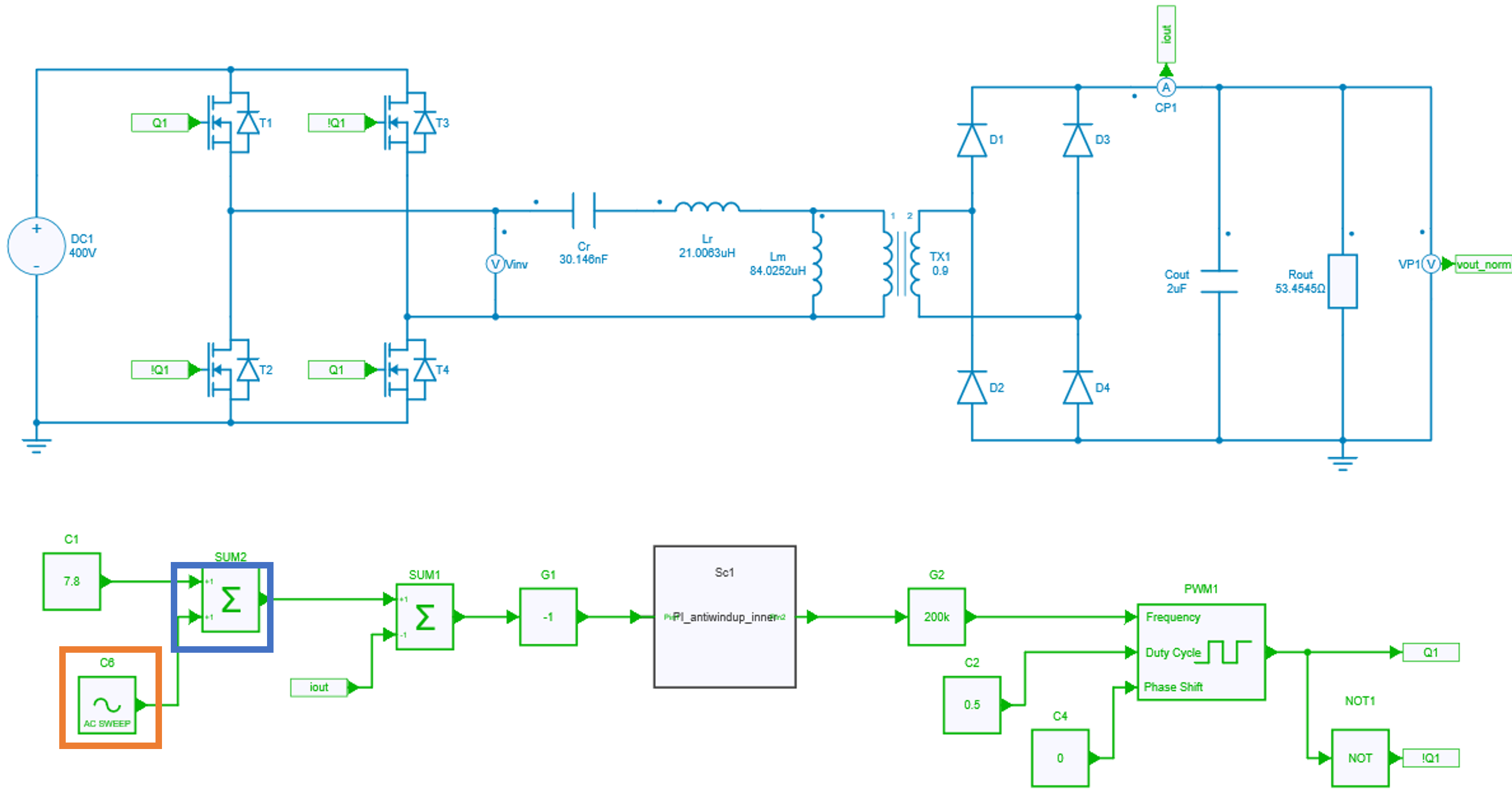
In this setup, since it is for outer loop, enable the scope ('VP1') which measures the voltage at the output.

Now, go again to the Test Bench in Simba GUI, and set up an AC Sweep Test Bench with the parameters as below:

testbench2

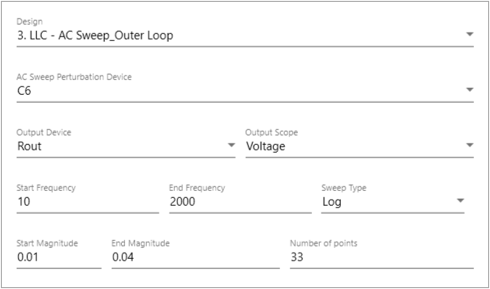
Further, test bench parameters can be tuned as per user's convenience. The result of the AC Sweep for outer loop is as shown below:

ACSweep2_result

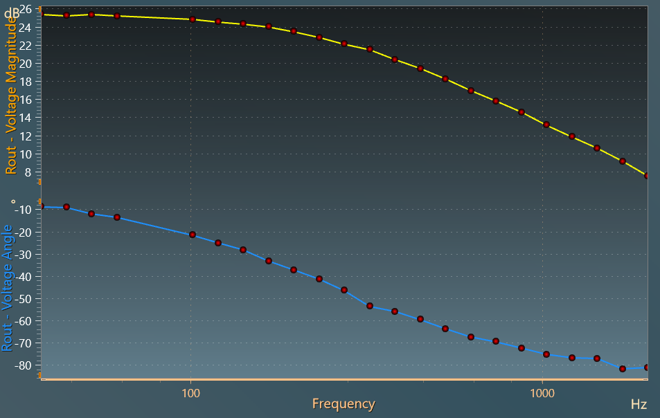
As it can be seen from the result, the angle data is regular and hence, there is no need to convert it into modulo 360°. Also, the data has to be saved in '.txt' format which can be done by using the code as given below:

df = pd.DataFrame({'Frequency': frequency_sim1, 'Amplitude': mag_sim1, 'Phase': phase_sim1 })
SweepOuter_txt = "SweepOuter.txt"
df.to_csv(SweepOuter_txt, sep='\t', index=False)
print(f"Data has been exported to {SweepOuter_txt}")

Tuning of outer loop using SmartCtrl

Again the file generated in above step can directly be imported in SmartCtrl to tune the controller. The steps mentioned below must be followed:

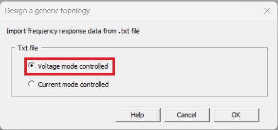
Launch SmartCtrl, 'Initial Dialog' window will be popped up and click on 'Import frequency response data from txt file' option at the bottom left of this window.
In the next window, select 'Voltage mode controlled' and click 'OK'. Further , provide path to the AC Sweep data in .txt file and give input as 420 in 'Vo(V)' tab, 200K in 'Fsw(Hz)' tab and click on 'OK'. This is becuase the nominal output voltage is 420 Volts and the switching frequency is 200 kHz.

SC6

Further in next window, select 'Isolate V.sensor' under 'sensor' tab, provide value to 'Vref(V)' tab as 1 and click on 'Calculate Gain' tab to re-calculate the gain for the entered set value, then click on 'OK'. Further, it will enable 'Compensator' tab where 'PI' option has to be selected from the drop-down menu. In this 'PI' window, write '1' in Vp(V) tab, '0' in Vv(V) tab, '4u' in 'tr(s)' tab and click 'OK'. It will take back to the previous window.

SC7

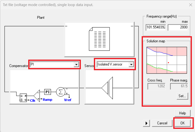
To proceed further, select 'Set...' tab which will show the solution map in a graph in white region, choose any point in the solution region and click 'OK'. This is the initial solution that is selected and it will take back to the previous window.
Finally, click 'OK' to reach to the final solution window where frequency and time domain analysis can be observed for the selected point in the solution map. In this case, the selected value is Kp = 64.637 and Ti(s) = 93.6610u which gives the Ki value as 690116.48 which is to be entered in the controller of outer loop.

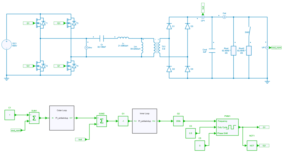
Complete closed loop simulation

In the final step, close the outer loop and run the simulation to check the results as in the attached model in design '4. LLC - Outer Loop' and shown in the figure below. If the selected value gives the satisfactory results, the controller values can be considered as the final value.

ClosedLoop

The result of the simulation is shown below:

Final_result

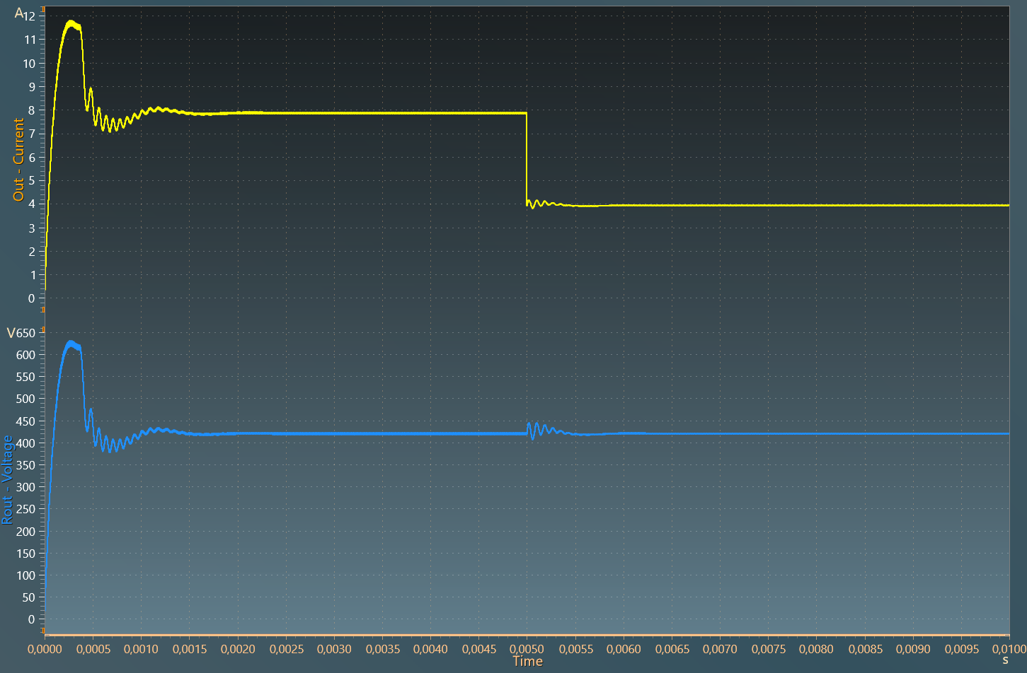
Hence, the closed loop design can easily be implemented for the full bridge LLC resonant converter using Simba and SmartCtrl.