How to Run Simulations with Parallel (Multiprocessing) Computing

This tutorial explores how to run parallel SIMBA simulations with multiprocessing. This is especially useful when a parameter sweep is done and a great number of simulations has to be run. Such examples are to get an efficiency map of a power converter for different operating points or to evaluate the influence of design parameters.

Note

Multiprocessing or multithreading are two different options for performing a parallel calculation. The choice of one of them will depend on the application and more precisely on the simulation time of a single job. Indeed, knowing that the creation of a process can take between 10 and 100 ms depending on the computer, the multiprocessing option will be more interesting when the simulation time of a single job is much longer.

The workflow is based on a combined use of the SIMBA python module and the multiprocessing python module.

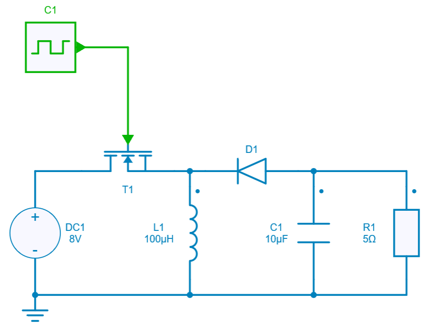
This tutorial considers a duty cycle sweep of the buck boost converter which can be loaded from the design examples to compute the mean value of the output voltage.

The python script and the Simba simulation file are also available on Github repository.

Python script architecture

It is advised to write the python script with different sections :

1. a first section where the circuit parameters and their sweep ranges are defined (in this tutorial: the duty cycle, its minimum and maximum value and the number of points),
2. a second section to define the functions - to be called in each process - and which:
   • loads the design and its circuit,
   • applies a parameter set to the circuit,
   • runs a simulation with this parameter set,
   • can perform post-processing computations (computes RMS values of the converter efficiency),
   • stores the results in a python list or other data structure.
3. a third section where the main part of the script distributes and run the calculations through the function defined in the 2nd section.

Detailed description of the python script

✔ Step 0: Load the required python modules

First, aesim.simba python module is loaded. For this tutorial the collection of design examples DesignExamples to get the buck boost converter and the License are also loaded.

Secondly, multiprocessing python module is loaded as well the tqdm module to get a progress bar in the terminal window.

Finally, numpy, matplotlib and datetime modules are loaded to respectively perform some calculations with arrays, plot and save a figure with a time stamp.

from aesim.simba import DesignExamples, License
import multiprocessing, tqdm #tqdm is for the progress bar
import numpy as np
import matplotlib.pyplot as plt
from datetime import datetime

First section: define parameters and their sweep range

✔ Step 1: Let's define here the maximum number of parallel simulations - based on the Parallel Simulation License (PSL) - the minimum and maximum values of the duty cycle and the number of points to be simulated.

number_of_parallel_simulations = License.NumberOfAvailableParallelSimulationLicense()
duty_cycle_min = 0
duty_cycle_max = 0.9
numberOfPoints = 200

Note

The variable named "number_of_parallel_simulations" allows setting automatically the number of available parallel simulation based on the license of each user.

Note that these lines can also be placed in the main script (3rd section described), but it is more readable to place them at the beginning of the script when a large number of parameters must be processed.

Second section: write the functions (which will be called by the main script) to run the simulation

✔ Step 2: Let's name this function run_job. It must have at least two types of arguments: input parameters and output variables. For this tutorial:

• inputs: the simulation number and the duty cycle value of the iteration (simulation),
• outputs: a list of the average output voltages to be calculated.

def run_job(simulation_number, duty_cycle, calculated_voltages):
    ...

First, the buck-boost converter from the design example collection is loaded, and then the PWM control block is found to set the duty cycle value:

    BuckBoostConverter = DesignExamples.BuckBoostConverter()   
    # Set duty cycle value
    PWM = BuckBoostConverter.Circuit.GetDeviceByName('C1')
    PWM.DutyCycle = duty_cycle
    ...

The simulation job is then created and run. If an error occured, the error message is plot for log purpose.

    # create job
    job = BuckBoostConverter.TransientAnalysis.NewJob()

    # Start job and log if error.
    status = job.Run()
    if str(status) != "OK": 
        print (job.Summary()[:-1])
        return; # ERROR 
    ...

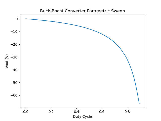
The simulation results are then stored into numpy arrays in order to compute the average value of the output voltage thanks to numpy average function. This average value is computed starting 2 ms to the end simulation time. The result is stored in a dedicated list which will contain the average values of all simulations and which is thus indexed with the simulation number.

    # Retrieve results
    t = np.array(job.TimePoints)
    Vout = np.array(job.GetSignalByName('Rload - Voltage').DataPoints)

    # Average output voltage for t > 2ms
    indices = np.where(t >= 0.002)
    Vout = np.take(Vout, indices)

    # Save Voltage in the results
    calculated_voltages[simulation_number] = np.average(Vout)

This ends this function writing.

✔ Step 3: Let's write now a wrapper function to call the first run_job function with only one argument (as a list). This helper function will be called by the object which will distribute the calculations in the main script.

def run_job_star(args):
    return run_job(*args)

Third section: Write the main script to distribute and run the calculations (processes)

✔ Step 4: This section is only called in the main thread of the main process and thus begins by:

if __name__ == "__main__":
    ...

✔ Step 5: Let's deal with the initialization step: the different duty cycles are calculated according to min and max values and the number of points to be simulated.

    duty_cycles = np.arange(duty_cycle_min, duty_cycle_max, duty_cycle_max / numberOfPoints)
    ...

Then, let's manage the input argument that will be sent to the simulation function run_job_star defined above. First, a manager object is created from the multiprocessing module to store the results. This object is a special list that several processes can access at the same time.

    manager = multiprocessing.Manager()
    calculated_voltages = manager.list(range(len(duty_cycles)))

Thus, the input argument named pool_args is a list of 200 (the number of simulation points) lists filled with:

• the simulation number,
• the duty cycle,
• the manager list of the output voltages to be calculated.

    pool_args = [[i, duty_cycles[i], calculated_voltages] for i in range(numberOfPoints)]

✔ Step 6: Let's now create the pool object which will distribute and run the calculations based on the number of available parallel simulation. The simulations are run with a progress bar through the tqdm object from the tqdm module.

    # Create and start the processing pool
    print("2. Running...")
    pool = multiprocessing.Pool(number_of_parallel_simulations)
    for _ in tqdm.tqdm(pool.imap(run_job_star, pool_args), total=len(pool_args)):
        pass

✔ Step 7: Last step deals with plotting results and save the figure:

    # Plot curve and save image.
    print("3. Plot output voltage vs duty cycle...")
    calculated_voltages = list(calculated_voltages)
    fig, ax = plt.subplots()
    ax.set_title("Buck-Boost Converter Parametric Sweep")
    ax.set_ylabel('Vout (V)')
    ax.set_xlabel('Duty Cycle')
    ax.plot(duty_cycles, calculated_voltages)
    path= "buck_boost_parametric_sweep_"+datetime.now().strftime("%m%d%Y%H%M%S")+".png"
    fig.savefig(path)

This last lines of code display the average value of the output voltage depending on the duty cycle as shown in the following figure:

This concludes this tutorial which highlights the benefit of parallel computing.