Efficiency map of a motor drive inverter with JMAG-RT model
Download python script for simulation
Download python script for displaying results
Download Python Library requirements
Motor drive inverter model
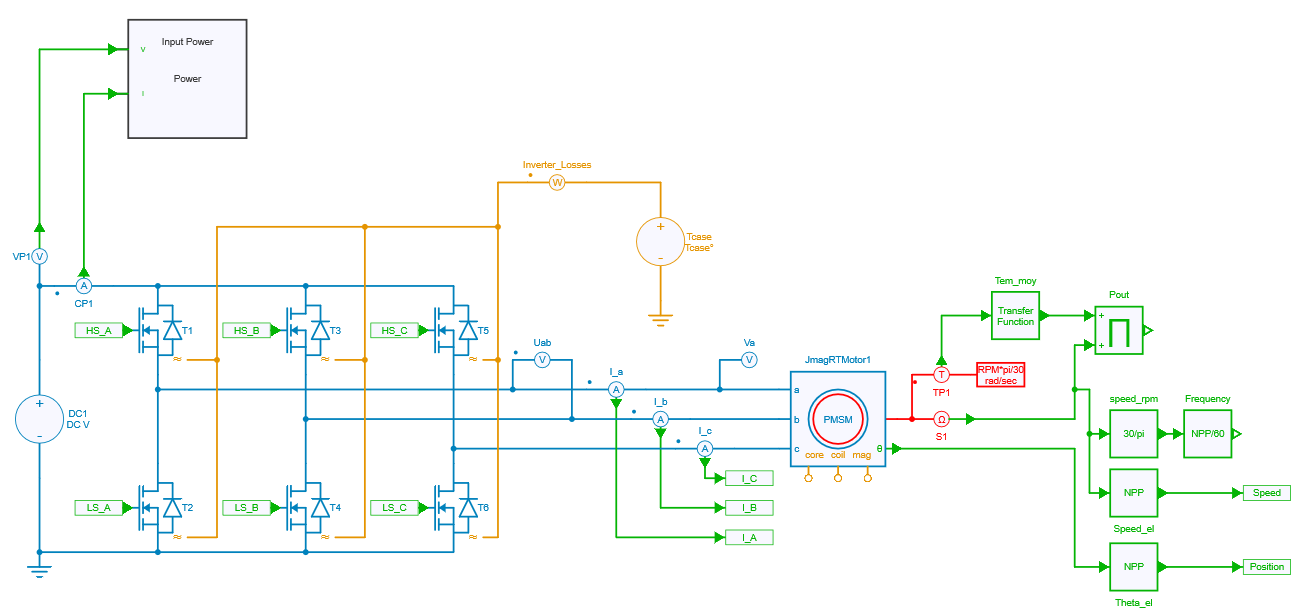
Inverter & motor model in SIMBA
The motor drive inverter model consists of a 3-phase 2-level voltage source inverter (VSI) that supplies a JMAG permanent magnet synchronous motor (PMSM). The PMSM is connected to a load that imposes a constant speed, meaning that the motor must be able to produce enough torque to maintain the desired speed.
Info
For detailed specifications of the motor, refer to JSOL website, where the PMSM model used for this simulation has been directly extracted. JMAG has the capability to provide real accurate machine model data by the use of .RTT file. Thus any JMAG user can extract .RTT file and implement a complete drive system in SIMBA. These specifications are summarized below:
| Motor specifications | |
|---|---|
| Model | 100k_D_D-I |
| Model Name | PMSM |
| Max. Power | 100 kW |
| DC Voltage | 500 V |
| RMS Current | 400 A |
| Number of Poles | 12 |
| Number of Slots | 72 |
| Number of Phases | 3 |
| Rotor | IPM |
| Stator (Outside Diameter) | 400 mm |
| Rotor (Outside Diameter) | 260 mm |
| Number of Turns | 3 |
| Height | 65 mm |
| Magnet | Neodymium sintered |
| Inertia Moment | 1.39e-1 kg / m² |
| Mass | 62.95 kg |
| Max. Current | 283 A |
| Calculation Results | JMAG Designer |
|---|---|
| Average torque | 177 N.m |
| Ld | 0.19 mH |
| Lq | 0.34 mH |
| Inductance | 0.18 mH |
| Torque Constant | 0.626 N.m / A |
Control
A DQ control has been implemented (described in another example which proposes this same principle of getting an inverter efficiency map but with an ideal PMSM).
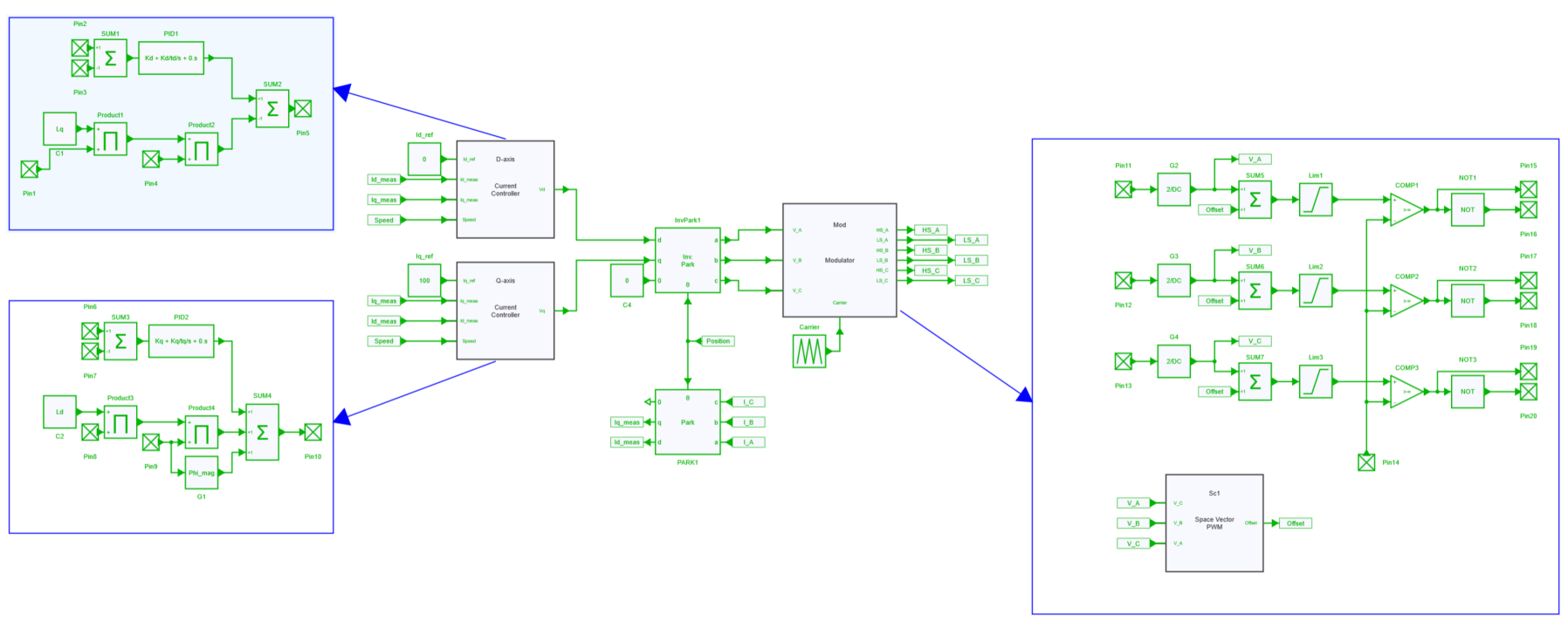
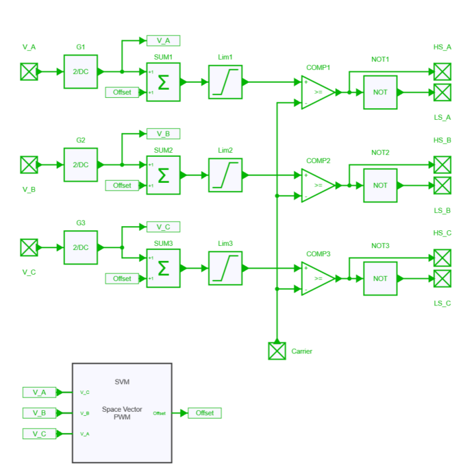
Yet, the modulation strategy considered here is a "carrier-based" space vector modulation (or MIN-MAX modulation).
Thermal modeling
To model the thermal performance of MOSFETs in an inverter, their package temperature is held constant and data is extracted from the .xml files provided by the manufacturer. In this particular case, Wolfspeed CAB006M12GM3 mosfets were used and can be downloaded here.
Python script
The first python script named efficiency_map_inverter_jmag.py uses the same architecture as in this example, which also uses the architecture presented in the tutorial Parallel (multiprocessing) computing and also available on Github repository).
Its primary objective is to run simulations at various operating points, such as different torque and speed levels, to obtain the losses of the drive in steady-state and generate an efficiency map. Yet, in this example the motor losses are also obtained thanks to the JMAG-RT model.
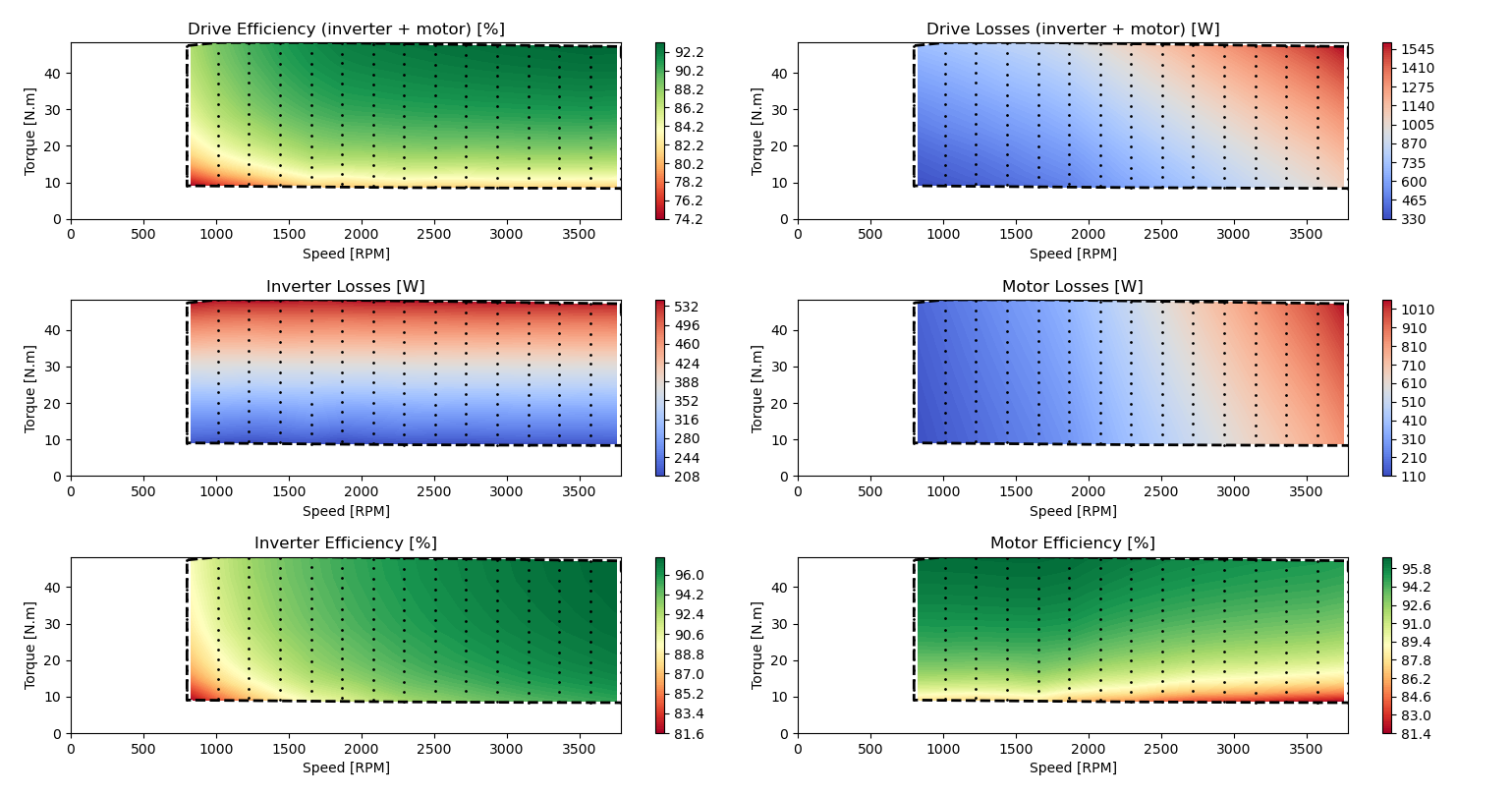
The second python script named efficiency_map_inverter_jmag_plot.py computes the inverter, the motor and the global efficiencies as described below and plots heatmaps of these losses and effiencies.
Drive efficiency:
Inverter efficiency:
Motor efficiency:
Results
The efficiency map was generated for a total of 225 speed / torque targets using the following simulation parameters:
case_temperature = 80           # Case temperature [Celsius]
Rg = 4.5                        # Gate resistance [Ohm]
switching_frequency = 50000     # Switching Frequency [Hz]
bus_voltage = 500               # Bus Voltage [V]
max_speed_ref = 4000            # [RPM]
max_current_ref = 100           # [A]

number_of_speed_points = 15     # Total number of simulations is number_of_speed_points * number_of_current_points
number_of_current_points = 15   # Total number of simulations is number_of_speed_points * number_of_current_points
relative_minimum_speed = 0.2    # fraction of max_speed_ref
relative_minimum_current = 0.2  # fraction of max_torque_ref
simulation_time = 0.5           # time simulated in each run

The figure below shows the resulting efficiency and loss map of the inverter, the motor and the global drive system: