Simulation Engine
This section explains how the simulation engine behind SIMBA works for users who would like to get a deeper understanding. Background theory might be necessary, so feel free to check the references or contact us if you have any questions.
Predictive Time-Step Solver
The Predictive Time-Step solver is a new type of transient solver developed to overcome the challenges of Power Electronics simulation:
- A typical converter model contains a wide spread of time-constants (Switching transients, Switching Frequency, Control System, Thermal...)
- Discontinuity events (Ex: Ideal Switch closing or opening)
- Model size ranging from a few nodes to a few thousand (Ex: multi-level converters or microgrids)
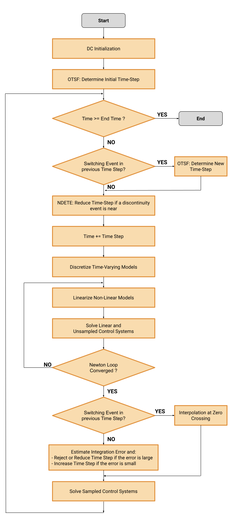
Our ambition is to be the best-in-class in terms of speed and accuracy for every use case. This section explains how we achieve this by detailing the different algorithms used by the Predictive Time-Step Solver. A simplified and high-level diagram of the Predictive Time-Step solver flow is available hereunder.
DC Initialization
A classic DC initialization is first performed to determine the initial state of the system. During the DC initialization, time-varying models (AC sources, inductors, capacitors...) are replaced by static models:
- AC sources are replaced by DC sources
- Inductors are replaced by current sources
- Capacitors are replaced by voltage sources
Optimal Time-Step Finder (OTSF)
Since typical converter models contain a wide spread of time constants that are continuously changing, it is obvious that fixed time-step solvers are not adapted. Fixed time-step solvers are good only when the smallest time-constant does not change during a simulation and this is rarely the case.
Variable time steps seem more adapted since the time step always matches the actual small time constants. The implementation of a variable time-step algorithm for power electronics simulation comes with two major challenges:
- What time step should be used at the beginning of the calculation?
- What time step should be used after a switching event?
Traditionally, the simulation starts with a small time-step defined by the user and is not impacted by switching events. This is a major problem because it leads to unnecessary small time steps (longer simulation time) and, worse, inadequate time steps when smaller time-constants are introduced by a switching event (switching transient, fault...).
For this reason, we have developed the OTSF algorithm that is called at the beginning of the transient simulation and after every switching event. This innovative algorithm analyzes each model and the entire circuit to determine what is the optimal time-step to use at a given time.
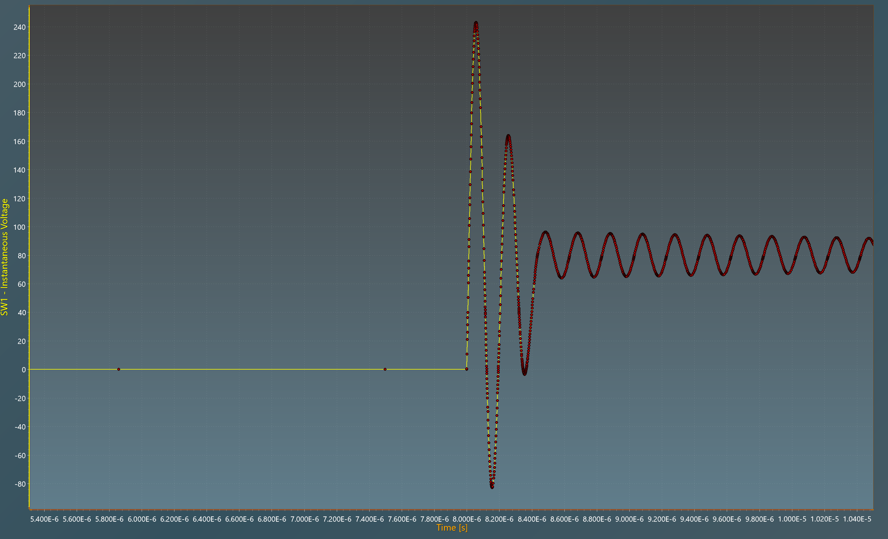
The waveform shown below shows the MOSFET voltage at turn-off in a forward converter. The high-frequency transients are due to the parasitic elements added to the model. After the switching event, the time step is optimal thanks to the OTSF. In this case, optimal means not too small (longer simulation) and not too large (inaccurate results).
Next Discontinuity Event Time Estimator (NDETE)
Another critical aspect required for reliable power electronic simulations is the discontinuity event time accuracy. In SIMBA, a discontinuity is a switching event or a control event like a gate or a comparator changing state. It is extremely important to simulate those events exactly when they are supposed to occur.
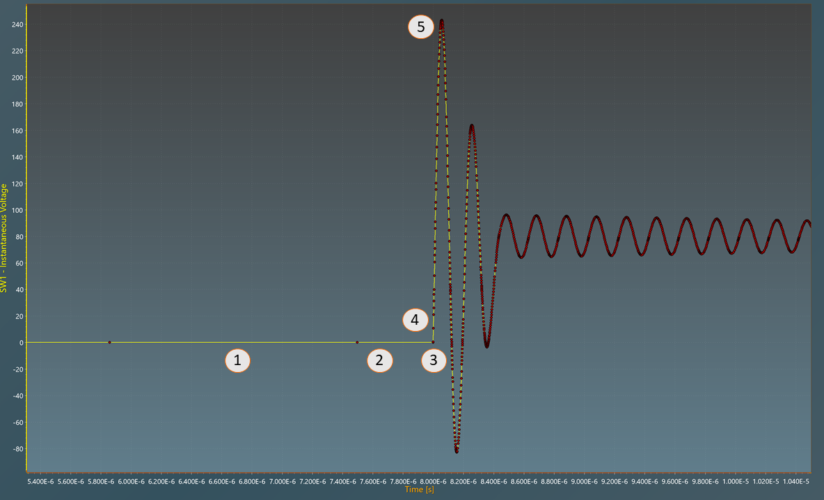
The NDETE is a machine learning algorithm running in parallel with the simulation. Its role is to analyze all the models and estimate when the next event will happen. If a discontinuity event will occur in the next time-step, it is automatically reduced to have a point just before the discontinuity event. A time step equal to the Min Time Step parameter is then used to simulate the discontinuity event. Finally, the OTSF algorithm is called to determine the new time-step after the discontinuity event. This is illustrated by the MOSFET voltage waveform shown previously:
- The Time Step is relatively large because the dynamic of the system is slow (≈2µs)
- The Time Step is reduced by the NDETE to calculate a point right before the discontinuity event (≈0.5µs)
- A Time-Step equal to the
Min Time Stepparameter is used to simulate the discontinuity event (=100ps) - The OTSF algorithm determines a new time-step to simulate the new time constants properly (≈2ns)
- The Time-Step evolves as the dynamic of the systems changes.
Zero-Crossing Switching Interpolation
When a switching device state changes after current or voltage zero-crossing, an interpolation algorithm is used to calculate a point exactly at the time of zero-crossing. This interpolation algorithm is mostly used for diodes switching and to prevent unphysical discontinuities.
The interpolated point is not shown to the user because the control system is not evaluated at the interpolated point.
Control Solver
The control solver is based on signal flow analysis. There are two types of control signals:
- Unsampled
The unsampled control signals are solved with the power solver. Therefore, there is no delay between the unsampled control devices and the power devices. This is important because SIMBA has a variable time step and some power devices (such as controlled sources) must be synchronized with the control solvers. This makes SIMBA a powerful tool for using average converter models.
- Sampled
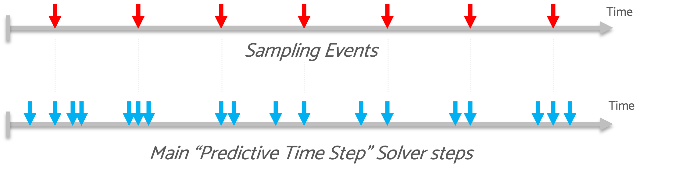
In some cases, it is necessary to build a control loop that behaves like a real digital controller: fixed sampling time and no iteration. For this reason, we have introduced the multi-time step solver that allows to calculate control devices at a fixed sampling rate.
"Sampling Time" parameter
All control devices have a sampling time parameter that is used to defined the sampling behovior and sampling time. Different values can be used to configure it:
-
auto: Inherit the sampling time of its source device (Unsampled by default).
-
none or 0: Unsampled. The system will be solved in the Newton loop.
-
Sampling Period: defined in seconds (Ex:
1u).
Multi Time-Step Solver
You can watch this video for more information on how SIMBA works with multiple time steps and how it handles sampling events.
Performance
Since a full time step is calculated at each sampling event, a small sampling period will result in a high computation time. The sampling time should only be used for digital controls and specific devices.
Algebraic loop
For performance reasons, algebraic loops are not supported but Memory models can be used to avoid them.
Stop at Steady-State
When Stop at Steady-State is enabled, the End Time parameter is not used, and the simulation stops when SIMBA detects the steady state. This feature is particularly useful during a parametric analysis because each run can have different time constants and the Stop at Steady-State feature ensures that each run will stop at its steady state. To determine if the steady state is reached, SIMBA analyzes the RMS value and the highest non-DC harmonics (if any) of all simulated state variables.
Modified Nodal Analysis
The Simulation Engine of SIMBA is based on the Modified Nodal Analysis. As compared with classic Nodal Analysis, Modified Nodal Analysis allows the modeling of ideal voltage sources and ideal switches. This is an obvious major advantage in terms of accuracy but also in terms of simulation speed since it keeps the main matrix well-conditioned.
State-Space or Modified Nodal Anlaysis
There is a lively discussion in the power electronics simulation software community on whether Nodal Analysis or State-Space Analysis is best suited for power electronics simulation.
State-Space analysis has certainly strong arguments in its favor. One of them is it does not introduce integration errors for linear systems. This means that the time-step can remain relatively large between switching events. On the other hand, the Nodal Analysis requires a smaller time-step to reach similar accuracy.
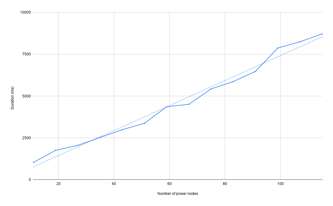
The main disadvantage of the State-Space analysis is it does not scale well. Indeed, the main matrix that needs to be inverted at each time step is not sparse. This causes a quadratic relation between system size (number of nodes) and computation time. On the contrary, the Nodal Analysis matrix is sparse (full of zeros) and if an efficient Sparse matrix solver is used, the computation time grows linearly with the number of nodes, which is a major advantage.
In Simba, a high-performance sparse matrix solver and a smart time-step control algorithm are used to simulate all the time-constants and discontinuity events of your power converter model as fast as possible, without compromising the accuracy and whatever the system size.
The following graph shows the relation between simulation time and model size. In SIMBA, simulation time grows linearly with the size of the simulated circuit.
References
- Najm, Farid N. Circuit Simulation. Wiley, 2010.
- Chen, Xiaoming. Parallel Sparse Direct Solver for Integrated Circuit Simulation. Springer, 2017.
- Introduction to Circuit Analyis