Electric Vehicle Battery Charger

This electric vehicle battery charger (EVBC) test case is comprised of a full bridge rectifier, an interleaved boost, and an LLC.

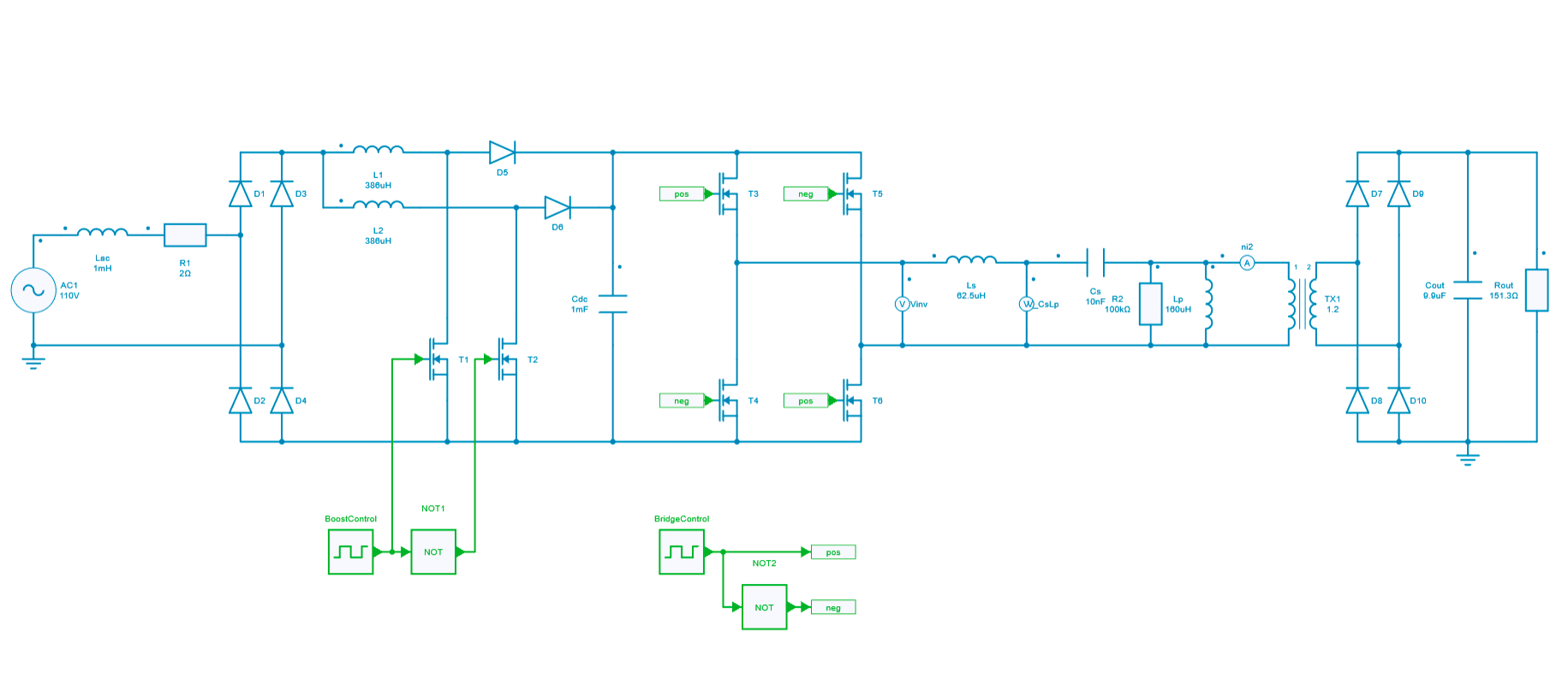
This test case demonstrates SIMBA's ability to simulate circuits composed of multiple high frequency switching converters requiring very small time steps.

Reference

H. Chalangar, T. Ould-Bachir, K. Sheshyekani and J. Mahseredjian, "Methods for the Accurate Real-Time Simulation of High Frequency Power Converters," in IEEE Transactions on Industrial Electronics, doi: 10.1109/TIE.2021.3114706.

Run Simulation

import numpy as np
import os
import time
import matplotlib.pyplot as plt
from aesim.simba import ProjectRepository, License

# Load Simba project
project = ProjectRepository(os.getcwd() + R"\isolated_battery_charger.simba")
mycvs = project.GetDesignByName('Design 1')

# Get the result object and solve the system
tic = time.process_time()
job = mycvs.TransientAnalysis.NewJob()
status = job.Run()
toc = time.process_time()
print('Elapsed time = ', toc - tic)
print('Number of points = ', np.shape(job.TimePoints)[0])

Elapsed time =  45.09375
Number of points =  9877910

PFC stage

# We'll keep only the first 2 period
index_2T = next(x[0] for x in enumerate(job.TimePoints) if x[1] > 2/60)
simba_time_2T = (job.TimePoints)[0:index_2T]

# Get results
simba_Cdc = job.GetSignalByName('Cdc - Voltage').DataPoints[0:index_2T]
simba_iL1 = job.GetSignalByName('L1 - Current').DataPoints[0:index_2T]
simba_iL2 = job.GetSignalByName('L2 - Current').DataPoints[0:index_2T]

#plot
fig, axs = plt.subplots(2,1,figsize=(15,10))
axs[0].set_ylabel('PFC Voltage (V)')
axs[0].set_xlabel('time (s)')
axs[0].plot(simba_time_2T,simba_Cdc, label ='PFC Voltage')
axs[0].legend(loc='upper left')

axs[1].set_ylabel('PFC Currents (A)')
axs[1].set_xlabel('time (s)')
axs[1].plot(simba_time_2T,simba_iL1, label ='iL1')
axs[1].plot(simba_time_2T,simba_iL1, label ='iL2')
axs[1].legend(loc='upper right')

plt.show();

LLC stage

# We'll keep only the point between 4.98ms and 5ms
index_4ms = next(x[0] for x in enumerate(job.TimePoints) if x[1] > 0.00498)
index_5ms = next(x[0] for x in enumerate(job.TimePoints) if x[1] > 0.005)
simba_time_0_5ms = (job.TimePoints)[index_4ms:index_5ms]

# Get results
simba_vInv = job.GetSignalByName('Vinv - Voltage').DataPoints[index_4ms:index_5ms]
simba_vCsLp = job.GetSignalByName('V_CsLp - Voltage').DataPoints[index_4ms:index_5ms]
simba_iLs = job.GetSignalByName('Ls - Current').DataPoints[index_4ms:index_5ms]
simba_iLp = job.GetSignalByName('Lp - Current').DataPoints[index_4ms:index_5ms]
simba_ni2 = job.GetSignalByName('ni2 - Current').DataPoints[index_4ms:index_5ms]
simba_vLp = job.GetSignalByName('Lp - Voltage').DataPoints[index_4ms:index_5ms]

#plot
fig, axs = plt.subplots(3,1,figsize=(15,15))
axs[0].set_ylabel('LLC Voltages (V)')
axs[0].set_xlabel('time (s)')
axs[0].plot(simba_time_0_5ms,simba_vInv, label ='Inverter Voltage')
axs[0].plot(simba_time_0_5ms,simba_vCsLp, label ='vCsLp Voltage')
axs[0].legend(loc='upper right')

axs[1].set_ylabel('LLC Currents (A)')
axs[1].set_xlabel('time (s)')
axs[1].plot(simba_time_0_5ms,simba_iLs, label ='iLs')
axs[1].plot(simba_time_0_5ms,simba_iLp, label ='iLp')
axs[1].plot(simba_time_0_5ms,simba_ni2, label ='ni2')
axs[1].legend(loc='upper right')

axs[2].set_ylabel('LLC Output Voltage')
axs[2].set_xlabel('time (s)')
axs[2].plot(simba_time_0_5ms,simba_vLp, label ='vLp')
axs[2].legend(loc='upper right')

plt.show();

Output Voltage

#get signals
simba_time = job.TimePoints
simba_vOut = job.GetSignalByName('Cout - Voltage').DataPoints

# figure
fig, ax = plt.subplots(figsize=(15,5))
ax.set_title("PFC voltages")
ax.set_ylabel('Voltage (V)')
ax.set_xlabel('time (s)')
ax.plot(simba_time,simba_vOut, label ='Output Voltage')
ax.legend(loc='upper left')
plt.show();